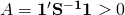
The concept of an “efficient frontier” was developed by Harry Markowitz in the 1950s. The efficient frontier shows us the minimum risk (i.e. standard deviation) that can be achieved at each level of expected return for a given set of risky securities.
Of course, to calculate the efficient frontier, we need to have an estimate of the expected returns and the covariance matrix for the set of risky securities which will used to build the optimal portfolio. These parameters are difficult (impossible) to forecast, and the optimal portfolio calculation is extremely sensitive to these parameters. For this reason, an efficient frontier based portfolio is difficult to successfully implement in practice. However, a familiarity with the concept is still very useful and will help to develop intuition about diversification and the relationship between risk and return.
In this post, I’ll demonstrate how to calculate and plot the efficient frontier using the expected returns and covariance matrix for a set of securities.
In a future post, I’ll demonstrate how to calculate the security weights for various points on this efficient frontier using the two-fund separation theorem.
In order to calculate the efficient frontier using n assets, we need two inputs. First, we need the expected returns of each asset. The vector of expected returns will be designated . The second input is the variance-covariance matrix for the n assets. This covariance matrix will be designated as . We also need a unity vector ( ) with the same length as the vector .
Once we have this information, we can run the following calculations using a matrix based mathematical program such as Octave or Matlab.

Using these values, the variance ( ) at each level of expected return ( ) is given by this equation:
You can see from the equation, that the efficient frontier is a parabola in mean-variance space.
Using the standard deviation ( ) rather than the variance, we have:
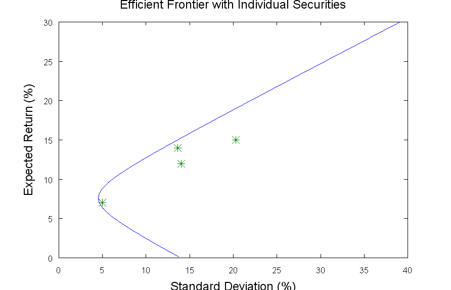
As an example, lets consider four securities, A,B,C and D, with expected returns of 14%, 12%, 15%, and 7%. The expected return vector is:
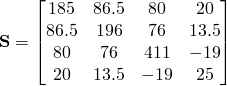
The covariance matrix for our example is shown below. In practice, the historical covariance matrix can be calculated by reading the historical returns into Octave or Matlab and using the cov(X) command. Note that the diagonal of the matrix is the variance of our four securities. So, if we take the square root of the diagonal, we can calculate the standard deviation of each asset (13.6%, 14%, 20.27%, and 5%).
The example script for computing the efficient frontier from these inputs is shown at the end of this post. It can be modified for any number of assets by updating the expected return vector and the covariance matrix.
The plot of the efficient frontier for our four assets is shown here:
Deriving the approach I have shown is beyond the scope of this post. However, for those who want to dive into the linear algebra, there are several excellent examples available online.
Derivation of Mean-Variance Frontier Equation using the Lagrangian (The Appendix B result is identical to what I show above, but the notation is a little different)
Octave Code:
This script will also work in Matlab, but I’ve chosen to use Octave since it is opensource and available for free.
% Mean Variance Optimizer % S is matrix of security covariances S = [185 86.5 80 20; 86.5 196 76 13.5; 80 76 411 -19; 20 13.5 -19 25] % Vector of security expected returns zbar = [14; 12; 15; 7] % Unity vector..must have same length as zbar unity = ones(length(zbar),1) % Vector of security standard deviations stdevs = sqrt(diag(S)) % Calculate Efficient Frontier A = unity'*S^-1*unity B = unity'*S^-1*zbar C = zbar'*S^-1*zbar D = A*C-B^2 % Efficient Frontier mu = (1:300)/10; % Plot Efficient Frontier minvar = ((A*mu.^2)-2*B*mu+C)/D; minstd = sqrt(minvar); plot(minstd,mu,stdevs,zbar,'*') title('Efficient Frontier with Individual Securities','fontsize',18) ylabel('Expected Return (%)','fontsize',18) xlabel('Standard Deviation (%)','fontsize',18)
in injection molding i have 2 defects (warpage&sink marks) they are controlled with variables(pressure&temperature) and i want to study the effect of the combination between these 2 variables on the 2 defects by using the efficient frontier .
please help me and tell me how can i do it and the equation needed thank you